IFRS9, PiTPD, and the Kalman Filter

Prior to the adoption of International Financial Reporting Standard 9 (IFRS9), provisioning were made only after exposures had turned delinquent. This “after-the-fact” shortcoming was heavily criticized for painting rosy pictures of the health of financial institutions before the 2008 Global Financial Crisis.

IFRS9 addressed the shortcoming by introducing the concept of expected credit loss (ECL). The calculation of ECL is quite daunting. One of the inputs that required in the calculation is the default probability of an obligor given a certain economic state. This is the so-called point-in-time PD (PiT PD).

One of the approaches of obtaining PiT PD is via Vasicek’s model. Specifically, Vasicek’s model postulates that PiT PD is given by

$P i T P D = N (\frac{N^{- 1} (T T C P D) - s \sqrt{ρ}}{\sqrt{1 - ρ}})$

where:

$T T C P D$ is the PD average over the long-run;
$N$ is the cumulative standard normal distribution;
$N^{- 1}$ is the inverse of the standard normal cumulative distribution;
$ρ$ is asset correlation;
$s$ is the common factor all obligors are subjected to. Further more, $s \sim N (0, 1)$ .

PiT PD is conditioned on $s$ . Therefore, $s$ can be interpreted as economic state. The challenge of getting $s$ is two folds:

$s$ has a specific form as required by Vasicek’s model, that is, $s \sim N (0, 1)$ . This is very different from the usual economic variables; and
$s$ is economic state, which is not directly observable.

This post shows how $s$ can be estimated using the Kalman Filter in R.

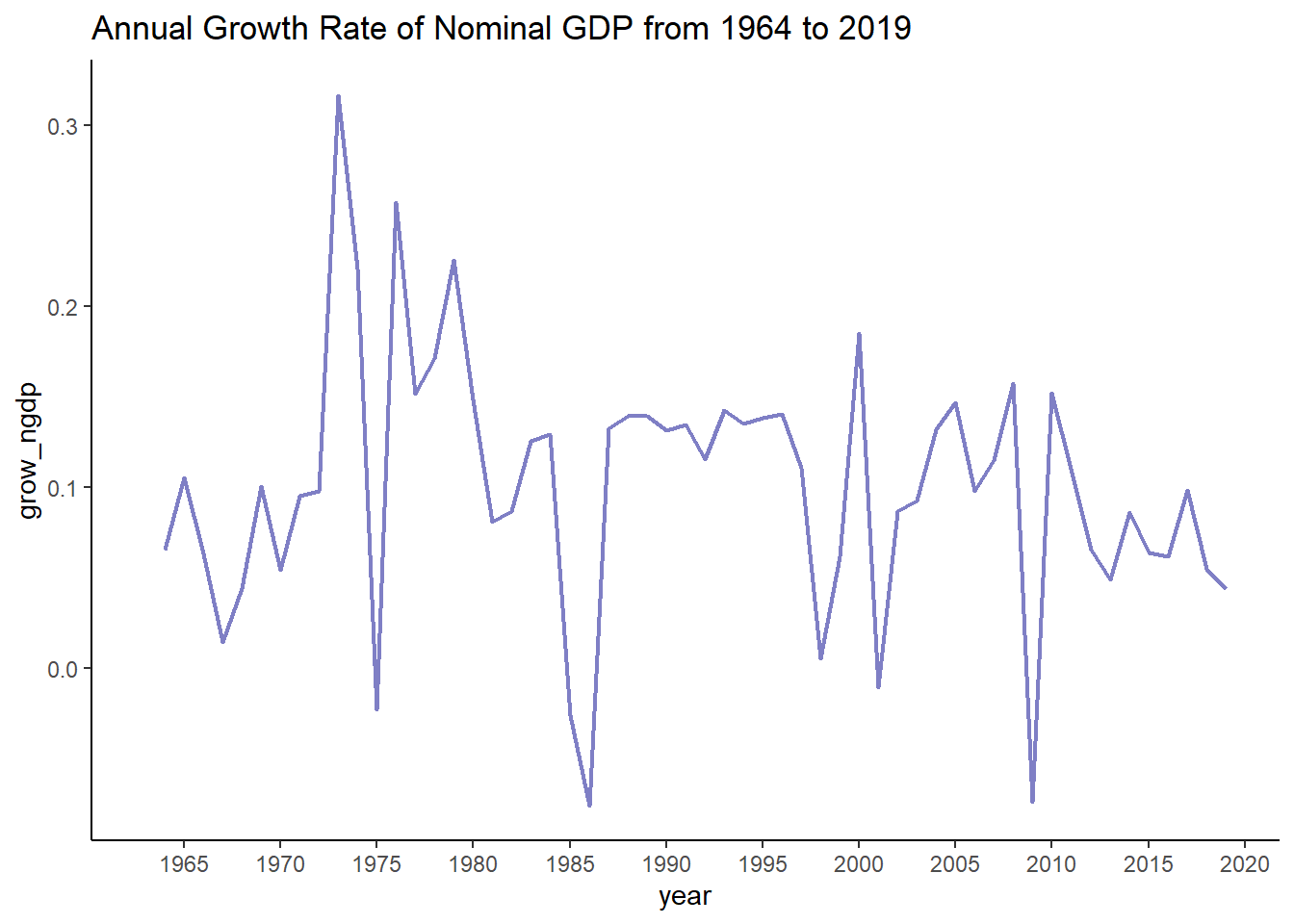
1.0 The Data

Due to the lack of long real GDP series in Malaysia (at the same constant prices), nominal GDP is used. The nominal GDP series spans 1963 to 2019. The analysis below uses the annual growth rate of the series.

2.0 The Model

The annual nominal GDP growth rate is observable. However, it may not reflect the true state of the economy. The true state of an economy is not directly observable.

Let $y_{t}$ be a variable that is directly observable and $x_{t}$ be a variable that is not directly observable. $x_{t}$ is called a state variable. To link these 2 variables together, a model in the state-space form can be written as:

$y_{t} = A x_{t} + v_{t}$ $x_{t} = Φ x_{t - 1} + w_{t}$

where $w_{t} \sim N (0, Q)$ and $v_{t} \sim N (0, R)$ .

The first equation is called the observation equation and the second equation is called the state equation. For the purpose of this post, the following conditions are imposed:

$y_{t}$ is the annual nominal GDP growth rate;
$x_{0} \sim N (0, 1)$ ;
$w_{t} \sim N (0, 1)$ ; and
$Φ = 1$

$A$ , $σ_{v}^{2}$ , and $x_{t}$ need to be estimated. $x_{t}$ is specified as a random walk process because its first difference is equal to $w_{t}$ , which is normally distributed with mean 0 and variance 1. The first-differenced $x_{t}$ can then be used to substitute $s$ in Vasicek’s model.

3.0 Estimation

The model in state-space form can be estimated using the Kalman Filter and the maximum likelihood approach. This is done below by using the astsa package in R.

The estimated values for $A$ and $σ_{v}$ are -0.07 and = 0.02, respectively.

 1
 2
 3
 4
 5
 6
 7
 8
 9
10
11
12
13
14
15
16
17
18
19
20
21
22
23
24
25
26
27
28
29


library(astsa)

y <- window(grow_ngdp, 1964, 2019)
num <- length(y)

# function to calculate likelihood
Linn <- function(parm) {

        # set up the parameters to be estimated        
        sigr <- parm[1]
        A <- parm[2]

        # set up all the parameters
        mu0 <- 0
        Sigma0 <- 1
        Phi <- 1
        cQ <- 1 # cQ is a lower triangle matrix from the Cholesky Decomposition of Q
        cR <- sigr # similar to cQ
        
        kf <- Kfilter0(num, y, A, mu0, Sigma0, Phi, cQ, cR)
        
        return(kf$like)
}        

# estimation 
init.par <- c(A = 0.2, sigr = 0.2) # initial parameters

est <- optim(init.par, Linn, NULL, method = 'BFGS', 
             hessian = TRUE, control = list(trace = 1, REPORT = 1, factr = 10^8))

 1
 2
 3
 4
 5
 6
 7
 8
 9
10
11
12
13
14
15
16
17
18
19
20


## initial  value -61.273853 
## iter   2 value -73.404880
## iter   3 value -96.008091
## iter   4 value -96.118280
## iter   5 value -99.259514
## iter   6 value -104.992422
## iter   7 value -110.249148
## iter   8 value -110.304797
## iter   9 value -110.955873
## iter  10 value -111.883887
## iter  11 value -113.783360
## iter  12 value -115.143845
## iter  13 value -115.826181
## iter  14 value -115.863203
## iter  15 value -115.885315
## iter  16 value -115.886933
## iter  16 value -115.886933
## iter  16 value -115.886933
## final  value -115.886933 
## converged

1
2


SE <- sqrt(diag(solve(est$hessian)))
round(cbind(estimate=est$par, SE), 2) 

1
2
3


##      estimate   SE
## A       -0.07 0.01
## sigr     0.02 0.01

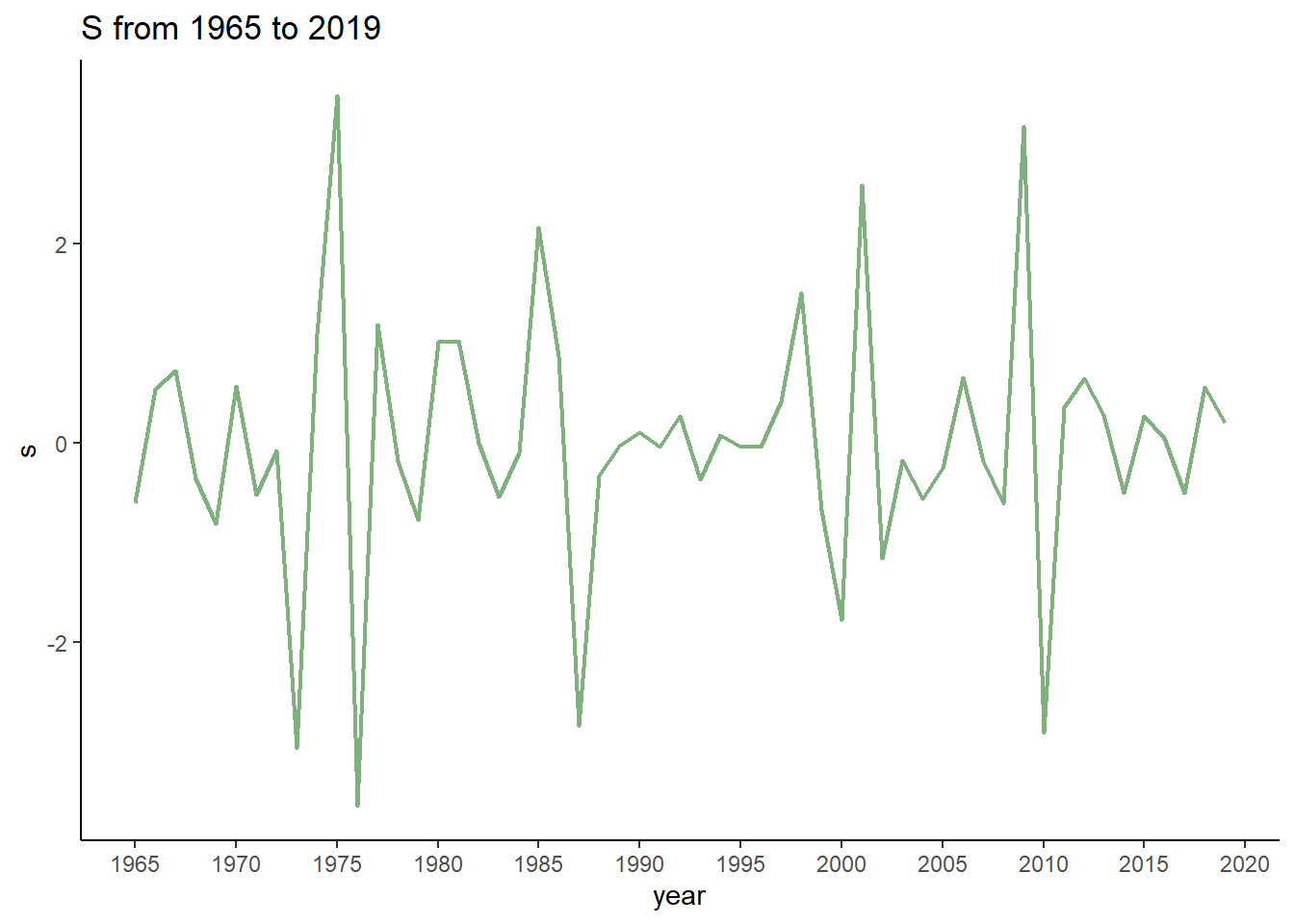
Next, the following codes are used to obtain $x_{t}$ and then first-difference is applied on $x_{t}$ . The resulting series is called $s$ .

$s$ can be selected based on the year and plugged into Vasicek’s model for the calculation of PiT PD (together with other inputs).

 1
 2
 3
 4
 5
 6
 7
 8
 9
10
11
12
13
14
15
16
17


# generation of x and s
mu0 <- 0
Sigma0 <- 1
Phi <- 1
cQ <- 1

A <- est$par[1]
cR <- est$par[2]

ks <- Ksmooth0(num, y, A, mu0, Sigma0, Phi, cQ, cR)

x <- as_tibble(ks$xf) %>% 
  pivot_longer(everything(), names_to = "var", values_to = "fil_x") %>%
  transmute(fil_x, year = seq(1964, 2019, length.out = 56))

state <- x %>%
  mutate(s = fil_x - dplyr::lag(fil_x))

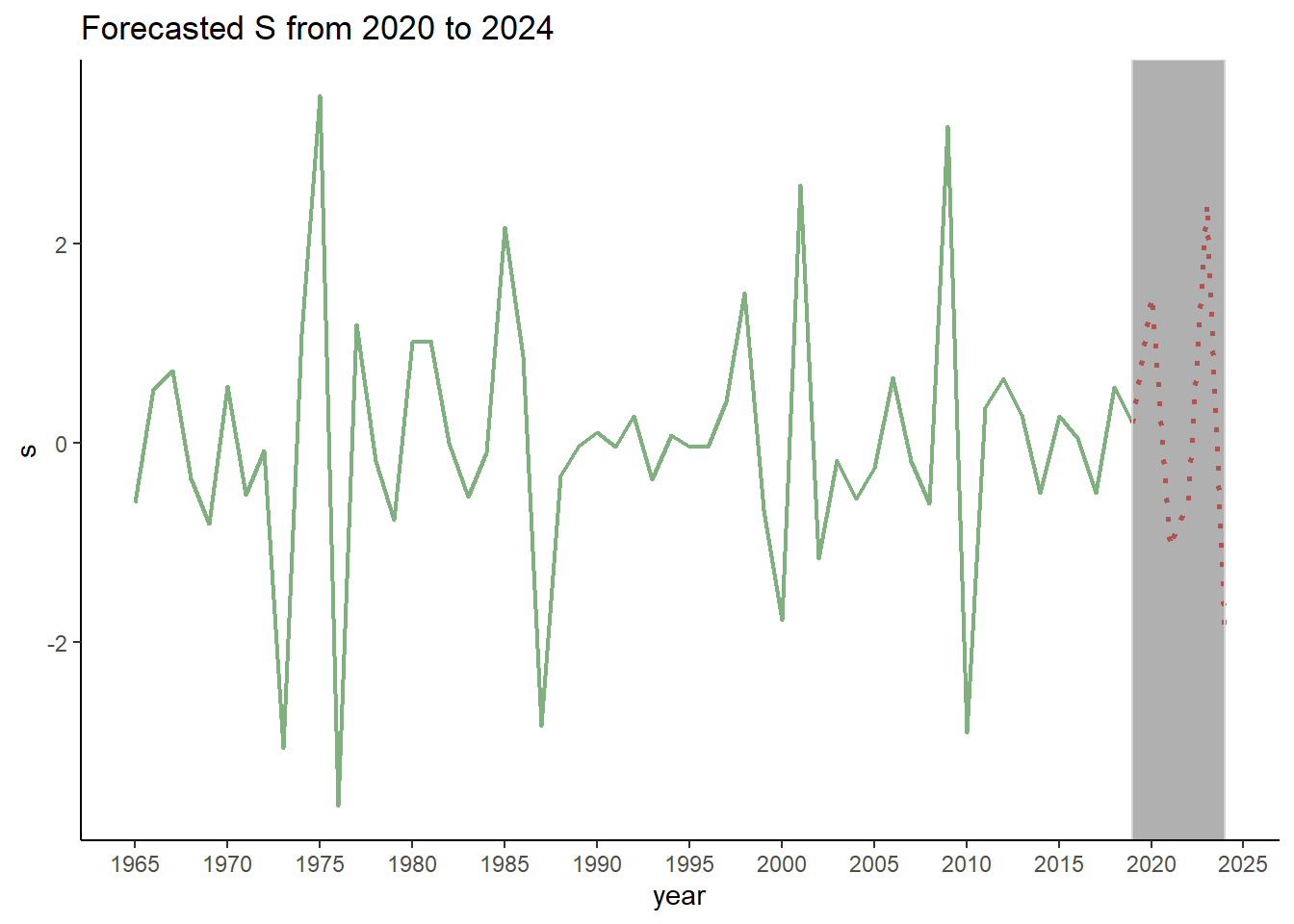
4.0 Forecasting

For the application in IFRS9, in-sample $s$ is insufficient as PiT PD is needed over the lifetime of an exposure. This suggests that forecasted values of $s$ are needed. As it turns out, the Kalman Filter has the forecasting algorithm built-in. This algorithm can be used, provided that the out-of-sample observable variable’s values are available. The codes below randomly generate out-of-sample $y_{t}$ and then generate the forecasted $s$ .

 1
 2
 3
 4
 5
 6
 7
 8
 9
10
11
12
13
14
15
16
17
18
19
20
21
22
23
24
25
26
27
28
29
30
31


set.seed(1234)
f_y <- rnorm(5, mean = 0, sd = 0.05)
num_ahead <- 5
f_x <- rep(0, 5) 

# select the last estimated values
x00 <- ks$xf[, , num] # last entry of estimated x value
P00 <- ks$Pf[, , num] # last entry of estimated error of x
Q <- t(cQ) %*% cQ  # estimated covariance matrix of w
R <- t(cR) %*% (cR) # estimated covariance matrix of v

for (m in 1:num_ahead){
  xp <- Phi %*% x00 
  Pp <- Phi %*% P00 %*% t(Phi) + Q
  sig <- A %*% Pp %*% t(A) + R 
  K <- Pp %*% t(A) %*% (1/sig)
  xf <- xp + K %*% (f_y[m] - A %*% xp)
  x00 <- xp
  P00 <- Pp - K %*% A %*% Pp
  f_x[m] <- xf
}

f_state <- as_tibble(f_x) %>%
  transmute(fil_x =value, 
            year = seq(2020, 2024, by = 1)
  )

all_state <- state %>%
  select(fil_x, year) %>%
  bind_rows(f_state) %>%
  mutate(s = fil_x - dplyr::lag(fil_x))

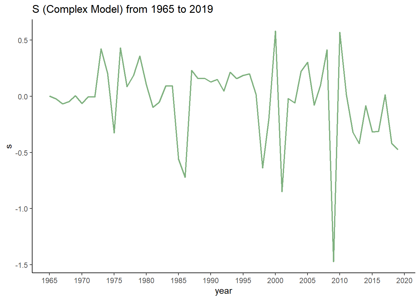
5.0 Complex Model

A much more complex model can be specified. Suppose that the observable variable $y_{t}$ follows an ARMAX(1,1) process and $x_{t}$ follows an ARIMA(1,1,0) process. Then, the model is:

$y_{t} = β_{1} + β_{2} s_{t} + β_{3} y_{t - 1} + β_{4} ϵ_{t - 1} + ϵ_{t}$ $x_{t} = x_{t - 1} + η_{t}$ $ϵ_{t} \sim N (0, σ_{ϵ}^{2})$ $η_{t} \sim N (0, 1)$

This model has been proposed by Chatterjee (2015). In state-space form, the model can be written as

$y_{t} = A x_{t}$ $x_{t + 1} = Φ x_{t} + Υ u_{t} + Θ v_{t}$

where:

$A = [\begin{matrix} 0 & 1 & 0 \end{matrix}]$ , $x_{t + 1} = [\begin{matrix} s_{t + 1} y_{t} β_{4} ϵ_{t} \end{matrix}]$ , $Φ = [\begin{matrix} 1 & 0 & 0 β_{2} & β_{3} & 0 0 & 0 & 0 \end{matrix}]$ , $Υ = [\begin{matrix} 0 & 0 & 0 0 & β_{1} & 0 0 & 0 & 0 \end{matrix}]$ , $u_{t} = [\begin{matrix} 0 1 0 \end{matrix}]$ , $Θ = [\begin{matrix} 1 & 0 & 0 0 & 1 & β_{4} 0 & β_{4} & 0 \end{matrix}]$ , and $w_{t} = [\begin{matrix} η_{t + 1} ϵ_{t} ϵ_{t - 1} \end{matrix}]$ .

There are 5 parameters (i.e $β_{1}$ to $β_{4}$ and $σ_{ϵ}^{2}$ ) to be estimated in this model.

 1
 2
 3
 4
 5
 6
 7
 8
 9
10
11
12
13
14
15
16
17
18
19
20
21
22
23
24
25
26
27
28
29
30
31
32
33
34
35
36
37
38
39
40
41
42
43


# complex model 
y <- window(grow_ngdp, 1964, 2019)
num <- length(y)

mu0 <- rep(0, 3)

Sigma0 <- diag(0, 3)  
Sigma0[1, 1] <- 1
Sigma0[2, 2] <- 0.01
Sigma0[3, 3] <- 0.01

Linn <- function(para) {
        b1 <- para[1]
        b2 <- para[2]
        b3 <- para[3]
        b4 <- para[4]
        sigQ <- para[5]
        
        A <- array(c(0, 1, 0), dim = c(1, 3, num))
        Gam <- 0      
        Phi <- matrix(c(1, b2, 0, 0, b3, 0, 0, 0, 0), 3)
        Ups <- matrix(c(0, 0, 0, 0, b1, 0, 0, 0, 0), 3)
        Theta <- matrix(c(1, 0, 0, 0, 1, b4, 0, b4, 0), 3)
        cQ <- diag(1, 3)
        cQ[2, 2] <- sigQ
        cQ[3, 3] <- cQ[2, 2]
        cR <- 0
        S <- matrix(c(0, 0, 0), 3)
        input <- matrix(c(rep(0, num), rep(1, num), rep(0, num)), num)
        
        kf <- Kfilter2(num, y, A, mu0, Sigma0, Phi, Ups, Gam, Theta, cQ, cR, S, input)

        return(kf$like) 
}

# estimation
init.par <- c(b1 = 0.001, b2 = 0.001, b3 = 0.001, b4 = 0.001, sigR = 0.01) # initial parameters

L <- c(0.001, 0.001, 0.001, -0.2, 0.001) # lower bound
U <- c(0.5, 0.5, 0.5, 0.2, 0.1) # upper bound

est <- optim(init.par, Linn, NULL, method = 'L-BFGS-B', lower = L, upper = U,
             hessian = TRUE, control = list(trace = 1, REPORT = 1, factr = 10^8))

 1
 2
 3
 4
 5
 6
 7
 8
 9
10
11
12
13
14
15
16


## iter    1 value -34.776305
## iter    2 value -111.577102
## iter    3 value -114.685828
## iter    4 value -118.151700
## iter    5 value -118.565339
## iter    6 value -119.767080
## iter    7 value -119.915127
## iter    8 value -120.004375
## iter    9 value -120.006625
## iter   10 value -120.014631
## iter   11 value -120.046926
## iter   12 value -120.057891
## iter   13 value -120.060584
## iter   14 value -120.060584
## final  value -120.060584 
## converged

1
2


SE <- sqrt(diag(solve(est$hessian)))
round(cbind(estimate=est$par, SE), 5) 

1
2
3
4
5
6


##      estimate       SE
## b1    0.09049  0.01710
## b2    0.00100  0.00353
## b3    0.11301  0.12956
## b4    0.03255 10.88302
## sigR  0.07095  0.02596

 1
 2
 3
 4
 5
 6
 7
 8
 9
10
11
12
13
14
15
16
17
18
19
20
21
22
23
24
25
26
27
28
29
30
31
32
33
34
35
36


# generation of x and s
mu0 <- rep(0, 3)

Sigma0 <- diag(0, 3)  
Sigma0[1, 1] <- 1
Sigma0[2, 2] <- 0.01
Sigma0[3, 3] <- 0.01

b1 <- est$par[1]
b2 <- est$par[2]
b3 <- est$par[3]
b4 <- est$par[4]
sigQ <- est$par[5]
        
A <- array(c(0, 1, 0), dim = c(1, 3, num))
Gam <- 0      
Phi <- matrix(c(1, b2, 0, 0, b3, 0, 0, 0, 0), 3)
Ups <- matrix(c(0, 0, 0, 0, b1, 0, 0, 0, 0), 3)
Theta <- matrix(c(1, 0, 0, 0, 1, b4, 0, b4, 0), 3)
cQ <- diag(1, 3)
cQ[2, 2] <- sigQ
cQ[3, 3] <- cQ[2, 2]
cR <- 0
S <- matrix(c(0, 0, 0), 3)
input <- matrix(c(rep(0, num), rep(1, num), rep(0, num)), num)
        
ks <- Ksmooth2(num, y, A, mu0, Sigma0, Phi, Ups, Gam, Theta, cQ, cR, S, input)

x <- tibble(fil_x = numeric(56), year = seq(1964, 2019, by = 1))

for (m in 1:num) {
  x$fil_x[m] <- ks$xf[1,1,m]
} 

state <- x %>%
  mutate(s = fil_x - dplyr::lag(fil_x))

From the graph below, it can be seen that downturns as suggested by relatively large negative values of $s_{t}$ are quite consistent with those generated by the simple model.

note

The forecasting algorithm for the complex model is different and is more complicated. Its analysis is omitted.

6.0 Conclusion

The Kalman Filter can be a handy tool for obtaining the required input for PiT PD calculation. However, for complex models, putting the models in state-space form could be a challenge. Another point worth mentioning is when estimating a complex model, the selection of initial values are critical.

Contents

1.0 The Data

2.0 The Model

3.0 Estimation

4.0 Forecasting

5.0 Complex Model

6.0 Conclusion