This is the final part of a 3-parts series.

6.0 Regression Analysis

The ground is now set for developing a credit scorecard. The technique, as widely documented in the literature, is based on logistic regression. To obtain a parsimonious logistic regression, one approach is to use the stepwise method. This method seeks to minimize the AIC by allowing variables to enter or to exit iteratively.

Each type of method has its own pros and cons and this will not be discussed here. Regardless of which type of method is used, it should be viewed as a tool that allows an analyst to keep the task more manageable. Significant amount of manual adjustments and judgments are still needed to be made in order to arrive at the final credit scorecard.

The codes below perform stepwise logistic regression analysis. The stepwise method produces a logistic regression with 6 variables (max_util_l6m is excluded). All 6 variables are significant at the 5% level and all coefficients are positive. To keep things simple, the resulting logistic regression is taken as final.

 1
 2
 3
 4
 5
 6
 7
 8
 9
10
# logistic regression
logistic <- glm(I(gb_flag == 0) ~ .,  # set the event as good, e.g. gb_flag==0
                family = binomial(),  # binomial is logistic regression
                data = dev_woe %>% select(-id)) # remove id column 
                                                                
# invoke stepwise regression based on AIC 
logistic_step <- step(logistic, direction = "both", trace = FALSE)

# print output
summary(logistic_step) 
 1
 2
 3
 4
 5
 6
 7
 8
 9
10
11
12
13
14
15
16
17
18
19
20
21
22
23
24
25
26
27
28
29
30
31
32
33
34
35
36
37
38
39
40
41
## 
## Call:
## glm(formula = I(gb_flag == 0) ~ pay_2_recode + pay_3_recode + 
##     pay_6_recode + avg_deq_l6m + max_deq_l6m + min_deq_l3m + 
##     min_deq_l6m + bill_amt2_util + bill_amt5_util + max_util_l3m + 
##     age_woe + pay_1_recode_woe + pay_4_recode_woe + pay_5_recode_woe + 
##     avg_util_l6m_woe, family = binomial(), data = dev_woe %>% 
##     select(-id))
## 
## Deviance Residuals: 
##     Min       1Q   Median       3Q      Max  
## -2.3131   0.4434   0.4973   0.5407   2.0459  
## 
## Coefficients:
##                  Estimate Std. Error z value Pr(>|z|)    
## (Intercept)       1.03541    0.06094  16.992  < 2e-16 ***
## pay_2_recode     -0.29873    0.04104  -7.280 3.34e-13 ***
## pay_3_recode     -0.33725    0.04501  -7.492 6.77e-14 ***
## pay_6_recode     -0.41495    0.04833  -8.586  < 2e-16 ***
## avg_deq_l6m       1.37781    0.18145   7.593 3.11e-14 ***
## max_deq_l6m      -0.23049    0.03691  -6.245 4.23e-10 ***
## min_deq_l3m       0.12436    0.06516   1.908   0.0563 .  
## min_deq_l6m       0.12222    0.07234   1.689   0.0911 .  
## bill_amt2_util   -0.34741    0.16290  -2.133   0.0330 *  
## bill_amt5_util    0.61995    0.10781   5.751 8.89e-09 ***
## max_util_l3m      0.36507    0.14629   2.495   0.0126 *  
## age_woe           0.62331    0.14728   4.232 2.31e-05 ***
## pay_1_recode_woe  0.89252    0.03171  28.146  < 2e-16 ***
## pay_4_recode_woe  0.42746    0.05038   8.484  < 2e-16 ***
## pay_5_recode_woe  0.44321    0.05262   8.423  < 2e-16 ***
## avg_util_l6m_woe  0.83584    0.14955   5.589 2.28e-08 ***
## ---
## Signif. codes:  0 '***' 0.001 '**' 0.01 '*' 0.05 '.' 0.1 ' ' 1
## 
## (Dispersion parameter for binomial family taken to be 1)
## 
##     Null deviance: 25433  on 23999  degrees of freedom
## Residual deviance: 21175  on 23984  degrees of freedom
## AIC: 21207
## 
## Number of Fisher Scoring iterations: 4

The output from the VIF analysis does not suggests any multi-collinearity issue.

1
2
# generate VIF 
vif(logistic_step, merge_coef = TRUE)
 1
 2
 3
 4
 5
 6
 7
 8
 9
10
11
12
13
14
15
16
17
##             variable   Estimate Std. Error z value Pr(>|z|)      gvif
##  1:      (Intercept)  1.0354118     0.0609 16.9918   0.0000        NA
##  2:     pay_2_recode -0.2987315     0.0410 -7.2799   0.0000  5.052485
##  3:     pay_3_recode -0.3372513     0.0450 -7.4923   0.0000  5.744389
##  4:     pay_6_recode -0.4149456     0.0483 -8.5855   0.0000  5.477218
##  5:      avg_deq_l6m  1.3778062     0.1814  7.5935   0.0000 52.220875
##  6:      max_deq_l6m -0.2304948     0.0369 -6.2452   0.0000  6.205415
##  7:      min_deq_l3m  0.1243624     0.0652  1.9085   0.0563  5.841826
##  8:      min_deq_l6m  0.1222177     0.0723  1.6894   0.0911  3.302808
##  9:   bill_amt2_util -0.3474052     0.1629 -2.1326   0.0330 14.702017
## 10:   bill_amt5_util  0.6199534     0.1078  5.7506   0.0000  4.938752
## 11:     max_util_l3m  0.3650659     0.1463  2.4954   0.0126 12.842162
## 12:          age_woe  0.6233068     0.1473  4.2321   0.0000  1.015499
## 13: pay_1_recode_woe  0.8925226     0.0317 28.1461   0.0000  3.232373
## 14: pay_4_recode_woe  0.4274605     0.0504  8.4841   0.0000  3.394157
## 15: pay_5_recode_woe  0.4432148     0.0526  8.4231   0.0000  3.429983
## 16: avg_util_l6m_woe  0.8358393     0.1495  5.5891   0.0000  6.765641

7.0 Scorecard Creation, Scaling, and Validation

Lastly, with the regression obtained, a credit scorecard can be created and validation exercise can be conducted.

The scaling used in this post is:

  • at score of 500, the good bad odd is 100 and;
  • the point of double odds (PDO) is 30. Moreover, the base score (i.e. intercept of the regression) is distributed evenly across the 6 variables.

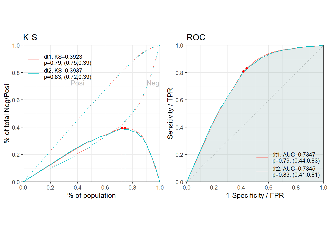
The package scorecard can generate a full-blown report that contains variables statistics, score distribution, scaling information, performance indicators and validation results.

Danger

In the codes below, PDO has to be set as -30. This is because positive = 0. And since positive = 0, anything that labeled as good in the report are actually referring to bad, and anything that labeled as bad are actually referring to good. Likewise, bad rate should be interpreted as good rate.

 1
 2
 3
 4
 5
 6
 7
 8
 9
10
11
12
13
14
15
16
17
18
19
20
21
22
## scorecard creation

# select the variables in the final regression
dev_final <- dev %>%
  select(id, gb_flag, age, avg_deq_l3m, pay_1_recode, pay_4_recode, pay_5_recode, avg_util_l6m)

var_select <- c("age", "avg_deq_l3m", "pay_1_recode", "pay_4_recode", "pay_5_recode", "avg_util_l6m")

breaks_list <- list(age = c("25", "45"), 
                    avg_deq_l3m = c("0.67",  "2"), 
                    pay_1_recode = c("1", "2"), 
                    pay_4_recode = c("1"), 
                    pay_5_recode = c("2"),
                    avg_util_l6m = c("0.45", "0.83")
                    )

bins <- woebin(dev_final, 
               y = "gb_flag", 
               x = var_select,
               positive = 0, 
               method = "freq", 
               breaks_list = breaks_list)                                                                                            
1
## [INFO] creating woe binning ...
1
2
3
4
5
6
7
8
score_card <- scorecard(bins, 
                       logistic_step, 
                       points0 = 500, 
                       pdo = -30, # PDO must set as negative   
                       odds0 = 100, 
                       basepoints_eq0 = TRUE)                                                                                   
# display results
score_card 
 1
 2
 3
 4
 5
 6
 7
 8
 9
10
11
12
13
14
15
16
17
18
19
20
21
22
23
24
25
26
27
28
29
30
31
32
33
34
35
36
37
38
39
40
41
42
43
44
45
46
47
48
49
50
51
52
53
54
55
56
57
58
59
60
61
62
63
64
65
66
67
68
69
70
71
72
73
74
75
76
77
78
79
## $basepoints
##      variable bin woe points
## 1: basepoints  NA  NA      0
## 
## $pay_2_recode
## Empty data.table (0 rows and 13 cols): variable,bin,count,count_distr,good,bad...
## 
## $pay_3_recode
## Empty data.table (0 rows and 13 cols): variable,bin,count,count_distr,good,bad...
## 
## $pay_6_recode
## Empty data.table (0 rows and 13 cols): variable,bin,count,count_distr,good,bad...
## 
## $avg_deq_l6m
## Empty data.table (0 rows and 13 cols): variable,bin,count,count_distr,good,bad...
## 
## $max_deq_l6m
## Empty data.table (0 rows and 13 cols): variable,bin,count,count_distr,good,bad...
## 
## $min_deq_l3m
## Empty data.table (0 rows and 13 cols): variable,bin,count,count_distr,good,bad...
## 
## $min_deq_l6m
## Empty data.table (0 rows and 13 cols): variable,bin,count,count_distr,good,bad...
## 
## $bill_amt2_util
## Empty data.table (0 rows and 13 cols): variable,bin,count,count_distr,good,bad...
## 
## $bill_amt5_util
## Empty data.table (0 rows and 13 cols): variable,bin,count,count_distr,good,bad...
## 
## $max_util_l3m
## Empty data.table (0 rows and 13 cols): variable,bin,count,count_distr,good,bad...
## 
## $age
##    variable       bin count count_distr good   bad   badprob         woe
## 1:      age [-Inf,25)  2168  0.09033333  588  1580 0.7287823 -0.26366705
## 2:      age   [25,45) 17639  0.73495833 3711 13928 0.7896139  0.07047959
## 3:      age [45, Inf)  4193  0.17470833 1037  3156 0.7526830 -0.13914675
##         bin_iv   total_iv breaks is_special_values points
## 1: 0.006734044 0.01382605     25             FALSE     16
## 2: 0.003579285 0.01382605     45             FALSE     25
## 3: 0.003512724 0.01382605    Inf             FALSE     19
## 
## $pay_1_recode
##        variable      bin count count_distr good   bad   badprob        woe
## 1: pay_1_recode [-Inf,1) 18504    0.771000 2567 15937 0.8612732  0.5737853
## 2: pay_1_recode    [1,2)  2943    0.122625  995  1948 0.6619096 -0.5803045
## 3: pay_1_recode [2, Inf)  2553    0.106375 1774   779 0.3051312 -2.0751013
##        bin_iv  total_iv breaks is_special_values points
## 1: 0.21391743 0.8648336      1             FALSE     45
## 2: 0.04764138 0.8648336      2             FALSE      1
## 3: 0.60327484 0.8648336    Inf             FALSE    -57
## 
## $pay_4_recode
##        variable      bin count count_distr good   bad   badprob        woe
## 1: pay_4_recode [-Inf,1) 21158   0.8815833 3806 17352 0.8201153  0.2650088
## 2: pay_4_recode [1, Inf)  2842   0.1184167 1530  1312 0.4616467 -1.4058353
##        bin_iv  total_iv breaks is_special_values points
## 1: 0.05735741 0.3616306      1             FALSE     28
## 2: 0.30427319 0.3616306    Inf             FALSE     -3
## 
## $pay_5_recode
##        variable      bin count count_distr good   bad   badprob        woe
## 1: pay_5_recode [-Inf,2) 21595   0.8997917 3992 17603 0.8151424  0.2316568
## 2: pay_5_recode [2, Inf)  2405   0.1002083 1344  1061 0.4411642 -1.4885586
##        bin_iv  total_iv breaks is_special_values points
## 1: 0.04517924 0.3354879      2             FALSE     27
## 2: 0.29030861 0.3354879    Inf             FALSE     -6
## 
## $avg_util_l6m
##        variable         bin count count_distr good   bad   badprob        woe
## 1: avg_util_l6m [-Inf,0.45) 14337   0.5973750 2621 11716 0.8171863  0.2452793
## 2: avg_util_l6m [0.45,0.83)  6103   0.2542917 1546  4557 0.7466820 -0.1711267
## 3: avg_util_l6m [0.83, Inf)  3560   0.1483333 1169  2391 0.6716292 -0.5365572
##         bin_iv   total_iv breaks is_special_values points
## 1: 0.033490587 0.09009968   0.45             FALSE     32
## 2: 0.007798286 0.09009968   0.83             FALSE     17
## 3: 0.048810811 0.09009968    Inf             FALSE      4
1
2
# compute score 
score <- scorecard_ply(dev_final, score_card, only_total_score = F)

The validation report will be saved in the work directory.

 1
 2
 3
 4
 5
 6
 7
 8
 9
10
11
12
13
14
15
16
17
18
19
## validation

# select the variables from OOT sample
oot_final <- oot %>%
  select(id, gb_flag, age, avg_deq_l3m, pay_1_recode, pay_4_recode, pay_5_recode, avg_util_l6m)

# generate reports
# good in the report is actually bad, whereas bad is actually good
report(list(dt1 = dev_final, dt2 = oot_final), 
       y = "gb_flag", 
       x = var_select, 
       breaks_list = breaks_list, 
       seed = NULL, 
       basepoints_eq0 = TRUE, 
       method = "freq", 
       positive = 0, 
       points0 = 500, 
       odds0 = 100,
       pdo = -30)
1
2
3
## [INFO] sheet1-dataset information
## [INFO] sheet2-model coefficients
## [INFO] sheet3-model performance

1
## [INFO] sheet4-variable woe binning

1
2
## [INFO] sheet5-scorecard
## [INFO] sheet6-population stability

1
2
## [INFO] sheet7-gains table
## [INFO] The report is saved as report_20201230_095053.xlsx

8.0 Conclusion

This post shows that a credit scorecard can be developed with ease in R using the package scorecard. The caveat is in the data set. The data set used in this post is small and clean, therefore, does not need a lot of cleaning and manipulations. The number of new variables that can be generated from the data set is also not huge.