Credit Scoring Development Using R - Part 2

This is the second part of a 3-parts series.

4.0 Univariate Analysis

4.1 Fine Classing

Fine classing is a technique that groups a variable’s values into a number of fine bins. Using these bins, a measure of the variable’s predictive power, known as information value (IV), can be computed. Also from these fine bins, further grouping can be carried out to result in coarse classing. As will be shown in the section below, bins from coarse classing are the bins that will be used in a credit scorecard.

Specifically, the fine classing technique used in this post is called the frequency method in the package scorecard. What this technique entails is grouping a variable’s values by having equal percentage of counts in each bin. This is a commonly used technique (see the note below). Following industry practice, the maximum number of fine bins is set at 20.

From this point on, the package scorecard will be used.

 1
 2
 3
 4
 5
 6
 7
 8
 9
10
11
12
13
14

library(scorecard)

# select all the variables for IV computation
var_list <- dev %>%
  select(-id, -gb_flag) %>%
  names()

# invoke the woebin function in package scorecard
fine_class <- woebin(dev, 
                    y = "gb_flag", 
                    x = var_list, 
                    positive = 1, # the value in gb_flag that indicates default
                    method = "freq", # frequency method
                    bin_num_limit = 20)  # the max number of fine bins

1

## [INFO] creating woe binning ...

1
2
3

# collect the IV of the variables
iv <- map_df(fine_class, ~pluck(.x, 10, 1)) %>%
  pivot_longer(everything(), names_to = "var", values_to = "iv")

The reports of the fine classing are contained in fine_class and can be viewed by typing fine_class and running it. Due to the massive amount of reports, only the first one is shown below.

 1
 2
 3
 4
 5
 6
 7
 8
 9
10
11
12
13
14
15
16
17
18
19
20
21
22
23
24
25
26
27

## $limit_bal
##      variable             bin count count_distr good bad   badprob        woe
##  1: limit_bal    [-Inf,30000)  1990  0.08291667 1272 718 0.3608040  0.6802441
##  2: limit_bal   [30000,50000)  1477  0.06154167  936 541 0.3662830  0.7039240
##  3: limit_bal   [50000,70000)  3358  0.13991667 2466 892 0.2656343  0.2352337
##  4: limit_bal  [70000,100000)  2369  0.09870833 1774 595 0.2511608  0.1596895
##  5: limit_bal [100000,140000)  2452  0.10216667 1853 599 0.2442904  0.1228206
##  6: limit_bal [140000,160000)  1512  0.06300000 1228 284 0.1878307 -0.2120476
##  7: limit_bal [160000,200000)  1973  0.08220833 1623 350 0.1773948 -0.2819782
##  8: limit_bal [200000,210000)  1202  0.05008333  987 215 0.1788686 -0.2719118
##  9: limit_bal [210000,270000)  2725  0.11354167 2259 466 0.1710092 -0.3263717
## 10: limit_bal [270000,360000)  2258  0.09408333 1941 317 0.1403897 -0.5599366
## 11: limit_bal [360000,430000)  1448  0.06033333 1235 213 0.1470994 -0.5054139
## 12: limit_bal   [430000, Inf)  1236  0.05150000 1090 146 0.1181230 -0.7582061
##          bin_iv  total_iv breaks is_special_values
##  1: 0.045171693 0.1785871  30000             FALSE
##  2: 0.036066804 0.1785871  50000             FALSE
##  3: 0.008242682 0.1785871  70000             FALSE
##  4: 0.002628082 0.1785871 100000             FALSE
##  5: 0.001593515 0.1785871 140000             FALSE
##  6: 0.002665805 0.1785871 160000             FALSE
##  7: 0.006024928 0.1785871 200000             FALSE
##  8: 0.003423424 0.1785871 210000             FALSE
##  9: 0.010999969 0.1785871 270000             FALSE
## 10: 0.024967126 0.1785871 360000             FALSE
## 11: 0.013268441 0.1785871 430000             FALSE
## 12: 0.023534628 0.1785871    Inf             FALSE

4.2 Initial Variables Removal

As discussed in the section above, new variables are derived because not all raw variables should be used directly. Numeric variables in amount such as balance, limit, payment are not advisable to be used because the variances in their values are large, rendering a credit scorecard unstable. Instead, these variables are converted into ratios (e.g. utilization rates) which are bounded below by zero and the maximum value should not be too far away from 100%.

Also discussed above is variables with a lot of missing values should be discarded. But this does not apply in this post because all variables have no missing values.

Lastly, variables with low predictive power as measured by IV are also removed (IV<0.02). However, since age’s IV is at the boarder line and it is preferable to have some demographic variables in a credit scorecard, age is kept.

With the above, the following variables are removed:

1. Low IV

• sex
• education
• marriage
• bill_amt1 to bill_amt5
• pay_amt6
• min_deq_l6m
• bill_amt1_util to bill_amt5_util
• min_util_l3m
• min_util_l6m

2. Variables in amount

• limit_bal
• pay_amt1 to pay_amt5
• bill_amt6

1
2
3

# keep the relevant variables
dev <- dev %>%
  select(id, age, gb_flag:max_util_l6m, avg_deq_l3m:min_deq_l3m, bill_amt6_util)

4.2 Variables Clustering

An analyst frequently faces thousands of variables. Even after filtering out variables with high missing values or with low IV values, hundreds of variables will still remain.

In addition to the IV and missing values criteria, variables clustering can be added to the variables reduction tool kit. The idea of variables clustering is to group similar variables into one cluster. Then, a few variables can be selected from each of the different clusters. An additional benefit that stems from variables clustering is that it could help reduce multi-collinearity among variables.

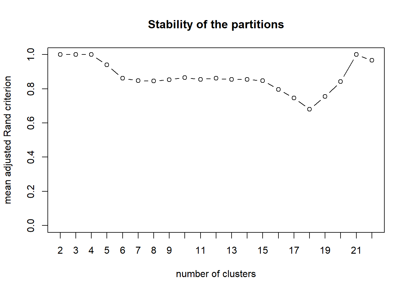
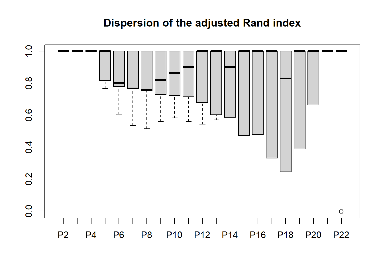
While it is not really applicable in this post as the number of variables is small, variables clustering is conducted for completeness. From the stability plot shown below, 4 clusters appear appropriate for the development sample. Hence, 4 cluster is set using cuttree. In the final output table below, the “x” column is cluster name. The application of this output is provided in the section below.

 1
 2
 3
 4
 5
 6
 7
 8
 9
10

library(ClustOfVar)

# perform variables clustering
tree <- dev %>%
  select(-id, -gb_flag) %>%
  hclustvar() 

# stability plot
set.seed(345)
stab <- stability(tree, B = 30) # B is bootstrapping sample. set B at 30 to 50 to reduce computing time 

1

boxplot(stab$matCR, main = "Dispersion of the adjusted Rand index")

1
2

# generate the final cluster output
clus <- cutree(tree, 4) 

4.3 Variables Reduction

One way to utilize the output from variables clustering is combining it with IV as follows:

In cluster 1, there is only one variable. Thus, age is short-listed. In cluster 2, the first 2 variables avg_deq_l3m and pay_1_recode are selected because they have the highest IVs in the cluster. Likewise for cluster 3, pay_4_recode and pay_5_recode are chosen. Finally, in cluster 4, the first 2 variables' IV are quite close and these 2 variables are of average utilization. Therefore, instead of choosing the first 2 variables, the first (avg_util_l6m) and the third (max_util_l6m) are short-listed.

5.0 Coarse Classing

To do coarse classing, it is necessary to go back to the fine classing reports generated previously, focusing solely on the short-listed variables.

One can use the fine classing reports directly for coarse classing. In this post, plots are used because they are easier for presentation. The plots are shown below one by one for the short-listed variables.

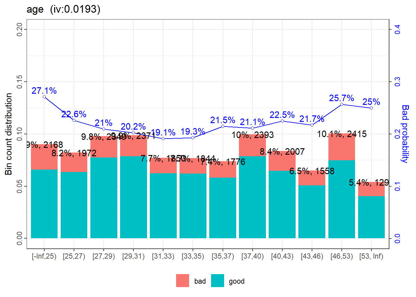
The first plot is for age. Referring to the plot, the bad rates of this variable is of U-shape. A plausible explanation that can be put forward is younger credit card holders are risky because of their lower income. On the other hand, old credit card holders are also risky because of having multiple loans, in retirement, or incurring heavy medical costs etc. For age, the coarse classing could be: a) <25, b)25 to <45, c) 45 and above. Note that the third bin is not starting from 46 as suggested by the plot. 45 is used just to make the bound nicer.

1
2

plot <- woebin_plot(fine_class_final)
plot[[1]]

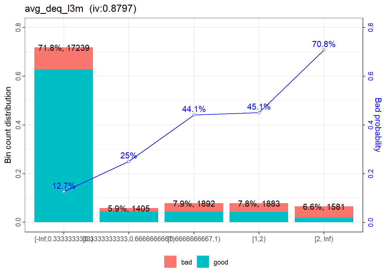
ave_deq_l3m is straight-forward. The bins with 44.1% and 45.1% bad rates are grouped together while others remain unchanged.

1

plot[[2]]

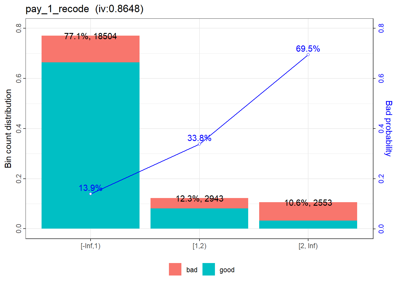
No further classing is necessary for pay_1_recode.

1

plot[[3]]

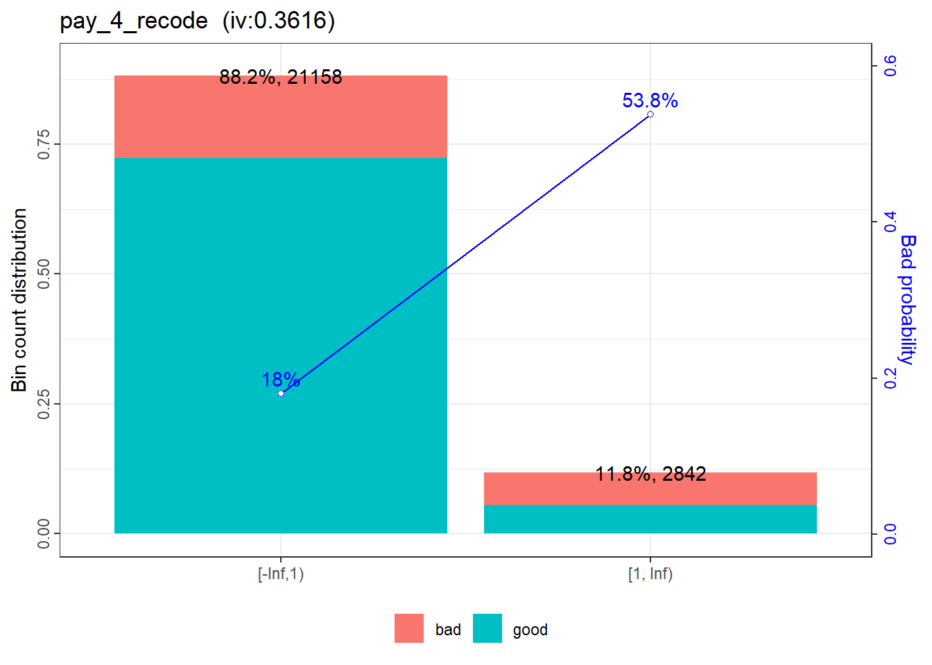
No further classing is necessary for pay_4_recode.

1

plot[[4]]

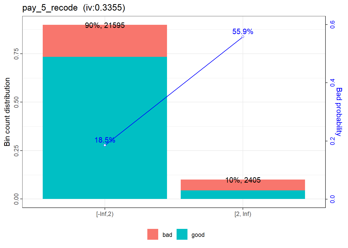
No further classing is necessary for pay_5_recode.

1

plot[[5]]

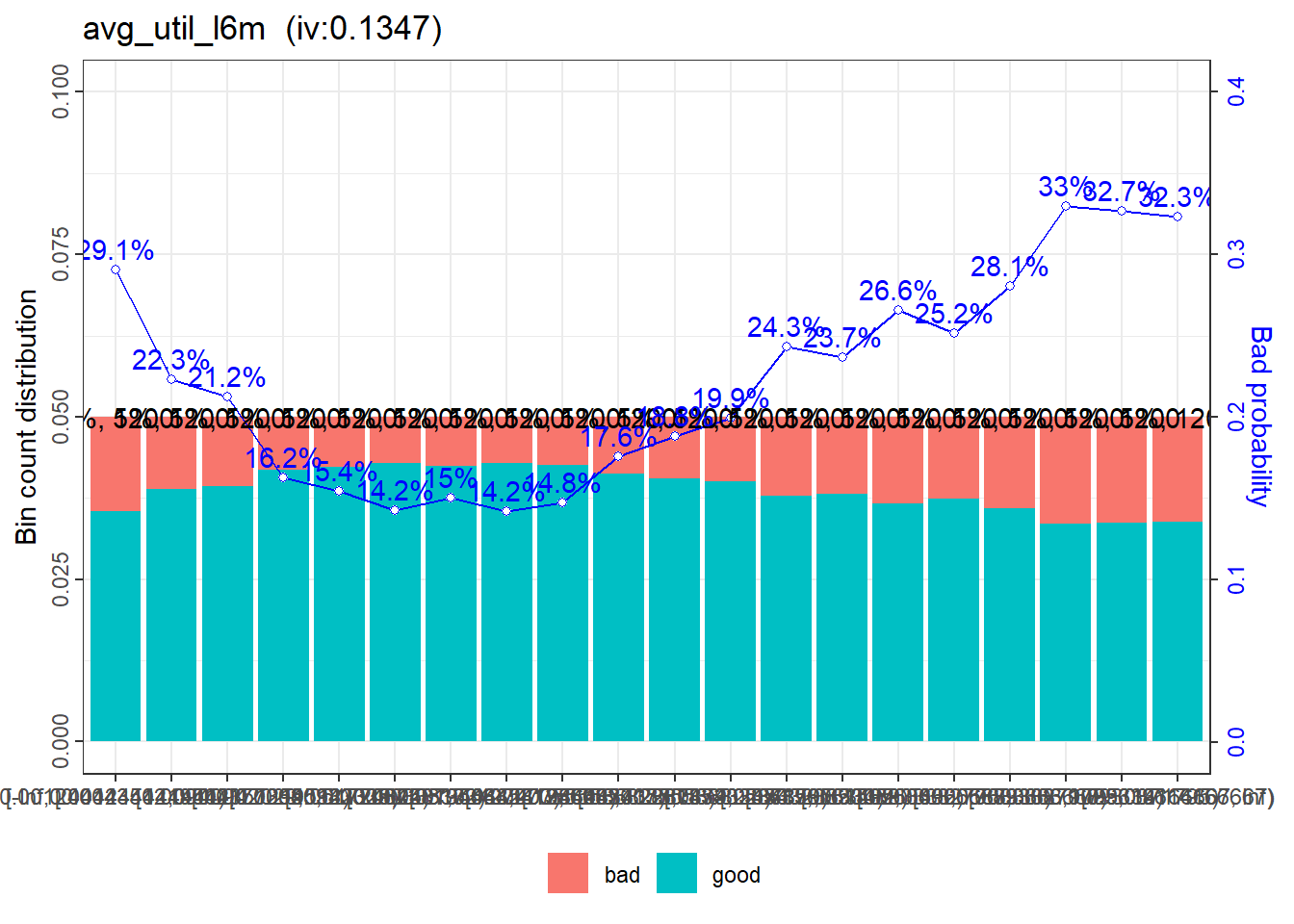
Utilization rates are expected to be monotonic in bad rates. That is, higher utilization rates associate with higher bad rates, or vice versa. Yet, this expectation is not consistent with what shown in the plot of avg_util_l6m. In the plot, it is those with lower utilization rates (i.e. first few bins) have higher bad rates.

For this variable, the coarse classing could be: a) <45%, b) 45% to <83%, and c) 83% and above. Note that minor tweaks are applied to the bounds of the bins. (Refer to the fine class report for the details of the bins.)

1

plot[[6]]

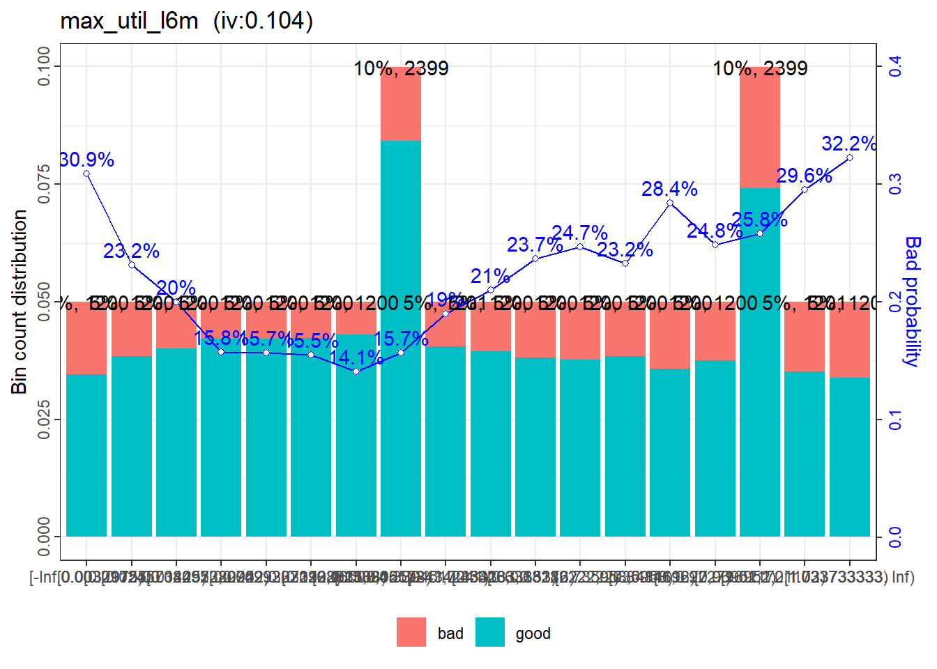
The situation of max_util_l6m is similar to avg_util_l6m. The coarse classing could be: a) <43%, b) 43% to <100%, and c) 100% and above. Minor tweaks are applied to the bounds of the bins.

1

plot[[7]]

The bounds resulted from the coarse classing of all short-listed variables can be saved into a list for future use.

1
2
3
4
5
6
7
8

breaks_list <- list(age = c("25", "45"), 
                    avg_deq_l3m = c("0.67",  "2"), 
                    pay_1_recode = c("1", "2"), 
                    pay_4_recode = c("1"), 
                    pay_5_recode = c("2"),
                    avg_util_l6m = c("0.45", "0.83"),
                    max_util_l6m = c("0.43", "1.00")
                    )

1
2
3
4
5
6
7

# set positive = 0
coarse_class <- woebin(dev, 
                       y = "gb_flag", 
                       x = short_var_list, 
                       positive = 0, 
                       method = "freq", 
                       breaks_list = breaks_list) # from coarse classing results

1

## [INFO] creating woe binning ...

1
2

# transform variables' values into WOE values
dev_woe <- woebin_ply(dev, coarse_class)  

1

## [INFO] converting into woe values ...