V-fold Cross Validation and Variables Derivation

In a predictive modeling project, one of the issues that an analyst always encounter is over what time period should a variable be derived. For example, should the analyst derive 3-month historical utilization rate to predict future default, or 6-month historical utilization rate is more appropriate.

Usually, when deriving variables over time period makes sense, the analyst would settle on 4 time periods: 3-month, 6-month, 9-month, and 12-month. And then, based on some predictive performance metrics such as information-value (IV) or AUC, one variant of the derivation is short-listed for the next stage of the model development process.

This approach is problematic. First, the selection of 3, 6, 9 and 12-month periods are judgmental, even though it is a common practice among practitioners. Second, when the variants are assessed using performance metrics, one particular variant could be better than the others simply due to over-fitting, which cannot be generalized to the yet-to-be-seen samples.

While tempting, the second point cannot be resolved by using the validation sample¹ that has been set aside for the evaluation of the final model. If the validation sample is used, then data leakage is introduced, which means that data outside the development sample is used to develop the model.

1.0 v-fold Cross Validation

This is an issue where cross validation can address. The figure below depicts the scheme of a 10-fold cross validation (v = 10). In essence, a 10-fold cross validation divides the development sample into 10 parts. In each fold, 9 parts are used for analysis and the remaining 1 part is used for testing. A testing part is technically a validation sample but the data does not come from the actual validation sample. Therefore, there is no data leakage in this approach. In addition, a testing sample covers different, non-overlapping region of the development sample as it iterates across different folds. Consequently, the performance metrics computed based on the testing samples will be free of over-fitting issue.

2.0 Data

The data is a data set on Taiwan’s credit card holders. It is sourced from UCI Machine Learning Center and a cleaned version can be obtained from Github.

 1
 2
 3
 4
 5
 6
 7
 8
 9
10

library(tidyverse)
library(janitor)

data <- read.csv("https://github.com/ngyongkad/scorecard/blob/main/Import%20Credit%20Card%20Defaults.csv?raw=true")  

# change the variable names to lower case 
# rename the default indicator and convert it into factor
data <- clean_names(data) %>%
  rename(gb_flag = default_payment_next_month) %>%
  mutate(gb_flag = as.factor(gb_flag))

To keep the analysis short and focus, only a few columns from the data set are selected.

 1
 2
 3
 4
 5
 6
 7
 8
 9
10
11
12
13
14
15
16
17

init_samp <- data %>%
 select(gb_flag, bill_amt1:bill_amt6)

obs_num <- nrow(init_samp)
var_num <- ncol(init_samp %>% select(bill_amt1:bill_amt6)) - 1 

# create a loop to calculate average bill_amt
amt <- as_tibble(matrix(NA, obs_num, var_num))

for (i in seq_along(1:var_num)) {
  j <- i + 2
  amt[, i] <- apply(init_samp[2:j], 1, mean)
  names(amt)[i] <- str_c("avg_bill_amt_last_", i + 1, "_mth")
}

# combine with the default indicator
init_samp_var <- bind_cols(amt, init_samp %>% select(gb_flag))

3.0 Sample Splitting

In this section, the initial sample is split and the folds of cross validation are generated.

1
2
3
4
5
6
7

library(tidymodels)

set.seed(123)
split <- initial_split(init_samp_var, prop = 0.75, strata = gb_flag)

# display the split
split

1
2

## <Analysis/Assess/Total>
## <22500/7500/30000>

The initial_split function in the tidymodels package splits the initial sample into a development sample of 22,500 credit card holders and a validation sample of 7,500 credit card holders. The vfold_cv function with option v = 10 creates 10 folds for cross validation from the development sample. 10 is a normally chosen value, but v can be higher or lower.

1
2
3
4
5
6
7
8
9

# development sample
devop <- training(split) 

# create 10-fold cross validation samples 
set.seed(456)
folds <- vfold_cv(devop, v = 10,  strata = gb_flag)

# display the 10 folds
folds

 1
 2
 3
 4
 5
 6
 7
 8
 9
10
11
12
13
14

## #  10-fold cross-validation using stratification 
## # A tibble: 10 x 2
##    splits               id    
##    <list>               <chr> 
##  1 <split [20.2K/2.3K]> Fold01
##  2 <split [20.2K/2.3K]> Fold02
##  3 <split [20.2K/2.3K]> Fold03
##  4 <split [20.2K/2.2K]> Fold04
##  5 <split [20.2K/2.2K]> Fold05
##  6 <split [20.2K/2.2K]> Fold06
##  7 <split [20.2K/2.2K]> Fold07
##  8 <split [20.3K/2.2K]> Fold08
##  9 <split [20.3K/2.2K]> Fold09
## 10 <split [20.3K/2.2K]> Fold10

4.0 10-fold Cross Validation

Cross validation is conceptually simple. But when it comes to implementation, it is not so straight forward as it involves many samples (i.e. folds) and multiple variables/models.

The analysis makes use of the scorecard and the tidymodels packages to:

1. scorecard: compute the IVs of the variants;
2. tidymodels: iterate over different folds and different variants.

As the codes can be hard to understand, it would be best to first describe how iterations work with the use of tidymodels. The function that is used is map. In the simplest form, map takes a list as the first argument and a function as the second argument. What map does is applying the function on each of the elements in the list. The following figure depicts the iteration. map2 works in the same way but takes 2 lists as inputs.

For each fold, the process is:

1. compute the IVs of the variants in the training sample;
2. save the break points that used for IV computations in step 1;
3. apply the break points on the testing sample and compute the IVs.

 1
 2
 3
 4
 5
 6
 7
 8
 9
10
11
12
13
14
15
16
17
18
19
20
21
22
23
24

## load the packages 
library(tidymodels)
library(scorecard)

## set up the necessary helper functions

# extraction function for pulling IV
extract_iv <- function(x) {
  map_df(x, ~ pluck(., 10, 1))  # 10 is the location of total IV 
}

# extraction function for pulling break points 
extract_blist <- function(x) {
  map(x, ~ pluck(., 11)) # 11 is the location of break list 
}

# cleaning function that removes "Inf" from break list
remove_inf <- function(x) {
  rmv <- function(x, y) {
    x[-y]
  }
  y <- map(x, length) # iterate over all of the elements in the list x
  map2(x, y, ~ rmv(.x, .y))
}

 1
 2
 3
 4
 5
 6
 7
 8
 9
10
11
12
13
14
15
16
17
18
19
20
21
22

# obtain the cross validated IV values from the training sample
train_cv <- folds %>%  
  mutate(cv_train    = map(splits, analysis), 
         woe_train   = map(cv_train, ~ woebin(., y = "gb_flag", method = "freq", bin_num_limit = 20, positive = "1")),
         iv_train    = map(woe_train, extract_iv),
         blist_long  = map(woe_train, extract_blist), 
         blist_short = map(blist_long, remove_inf) # pass the break points for use in the testing sample
        ) 

# obtain the cross validated IV values from the testing sample
test_cv <- train_cv %>% 
  select(splits, id, blist_short) %>%
  mutate(cv_test  = map(splits, assessment), 
         woe_test = map2(cv_test, blist_short, ~ woebin(.x, y = "gb_flag", method = "freq", positive = "1", breaks_list = .y)),
         iv_test  = map(woe_test, extract_iv))

# tidy the IVs from the testing sample
test_iv_summary <- test_cv %>% 
  select(id, iv_test) %>%
  unnest(cols = iv_test) %>%
  summarise(across(-id, mean, .names="{.col}_iv_mean")) %>%
  pivot_longer(everything(), names_to = "var", values_to = "iv_mean")

1
2
3
4
5

# visuallize the results 
test_iv_summary %>%
  mutate(var = str_remove_all(var, "bill_amt_|_iv_mean")) %>%
  ggplot(mapping = aes(x = var, y = iv_mean)) +
  geom_bar(fill = "darkblue", stat = "identity")

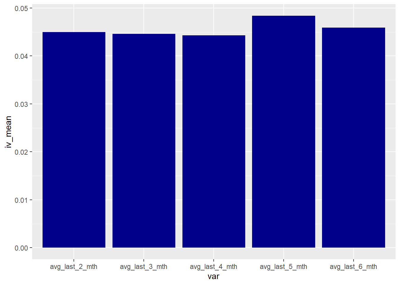
5.0 Conclusion

The analysis shows that the usual time periods used for variables derivations can be sub-optimal. The approach shown here essentially treats time period as a tuning parameter and use v-fold cross validation to determine the optimal parameter. In addition, v-fold cross validation eliminates any doubts on over-fitting and avoid data leakage. With some modifications, the approach can be applied in a wide range of applications.